Analyzing multi-gigabyte JSON files locally

I’ve had the pleasure of having had to analyse multi-gigabyte JSON dumps in a project context recently. JSON itself is actually a rather pleasant format to consume, as it’s human-readable and there is a lot of tooling available for it. JQ allows expressing sophisticated processing steps in a single command line, and Jupyter with Python and Pandas allow easy interactive analysis to quickly find what you’re looking for.

However, with multi-gigabyte files, analysis becomes quite a lot more difficult. Running a single jq command will take a long time. When you’re ~trial-and-error~iteratively building jq commands as I do, you’ll quickly grow tired of having to wait about a minute for your command to succeed, only to find out that it didn’t in fact return what you were looking for. Interactive analysis is similar. Reading all 20 gigabyte of JSON will take a fair amount of time. You might find out that the data doesn’t fit into RAM (which it well might, JSON is a human-readable format after all), or end up having to restart your Python kernel, which means you’ll have to endure the loading time again.

Of course, there’s cloud-based offerings that are based on Apache Beam, Flink and many others. However, customer data doesn’t go on cloud services on my authority, so that’s out. Setting up an environment like Flink locally is doable, but a lot of effort for a one-off analysis.

While trying to analyse files of this size, I’ve found two ways of doing efficient local processing of very large JSON files that I want to share. One is based on parallelizing the jq command line with GNU parallel, the other is based on Jupyter with the Dask library.

In the Beginning was the Command Line: JQ and Parallel

I try to find low-effort solutions to problems first, and most of the tasks I had for the JSON files were simple transformations that are easily expressible in jq’s language. Extracting nested values or searching for specific JSON objects is very easily accomplished. As an example, imagine having 20 Gigabytes of structures like this (I’ve inserted the newlines for readability, the input we’re actually reading is all on one line):

{
  "created_at": 1678184483,
  "modified_at": 1678184483,
  "artCode": "124546",
  "status": "AVAILABLE",
  "description": "A Windows XP sweater",
  "brandName": "Microsoft",
  "subArts": [
    {
      "created_at": 1678184483,
      "modified_at": 1678184483,
      "subCode": "123748",
      "color": "green",
      "subSubArts": [
        {
          "created_at": 1678184483,
          "modified_at": 1678184483,
          "code": "12876",
          "size": "droopy",
          "currency": "EUR",
          "currentPrice": 35
        },
        {
          "created_at": 1678184483,
          "modified_at": 1678184483,
          "code": "12876",
          "size": "snug",
          "currency": "EUR",
          "currentPrice": 30
        }
      ]
    },
    {
      "created_at": 1678184483,
      "modified_at": 1678184483,
      "subCode": "123749",
      "color": "grey",
      "subSubArts": [
        {
          "created_at": 1678184483,
          "modified_at": 1678184483,
          "code": "12879",
          "size": "droopy",
          "currency": "EUR",
          "currentPrice": 40
        },
        {
          "created_at": 1678184483,
          "modified_at": 1678184483,
          "code": "12876",
          "size": "snug",
          "currency": "EUR",
          "currentPrice": 35
        }
      ]
    }
  ]
}

A jq query like .subArts[]|select(.subSubArts[].size|contains("snug")) will give you all subarticles having a subsubarticle with a size of “snug”. Running a similar command on a 10-gigabyte JSON file took about three minutes, which isn’t great, especially when you’re impatient (like I happen to be).

Luckily, we can speed this up, if we have some information about the structure of the input file (we know the format is JSON, obviously). We’re using jq as a filter for single JSON objects, which means that we should be able to efficiently parallelize the search expression. Whenever I have to run shell commands in parallel, I reach for GNU parallel, which can handle shell commands, SSH access to remote servers for a DIY cluster, SQL insertion and lots more.

In this case, we know that our JSON objects in the file are delimited by a closing curly bracket followed by a newline, one JSON object per line. This means that we can tell parallel to run jq in parallel on these JSON objects with the --recend switch. Note that you could also tell parallel to interpret --recend as a regular expression, which would allow you to correctly split the pretty-printed example above with a --recend of ^}\n. This is probably substantially slower, I wouldn’t use a tool that spits out 10 gigabyte of pretty-printed JSON, and if necessary, I would just use jq -c to collapse it again.

Spawning a single jq process for every JSON object would not lead to a speedup (because executing new processes is expensive), which is why we tell parallel to collect complete objects into blocks, and pass those to a jq process. The optimal block size will depend on the size of the input file, the throughput of your disk, your number of processors, and others. I’ve had sufficient speedup with a block size of 100 megabyte, but choosing a larger block size would probably not hurt. Parallel can split up files in an efficient manner using the --pipe-part option (for the reasons as to why this is more efficient, see here), so we can use this to provide input to our parallel jq processes.

Finally, the worst part of every parallel job: Ordering the results. Parallel has lots of options for this. We want to keep our output in the original order, so we add the --keep-order argument. The default configuration, --group, would buffer input for each job until it is finished. Depending on your exact query, this will require buffering to disk if the query output can’t fit in main memory. This is probably not the case, so using --group would be fine. However, we can do slightly better with --line-buffer, which, in combination with --keep-order, starts output for the first job immediately, and buffers output for other jobs. This should require slightly less disk space or memory, at the cost of some CPU time. Both will be fine for “normal” queries, but do some benchmarking if your query generates large amounts of output.

Finally, provide the input file with --arg-file. Putting it all together, we get our finished command line:

parallel -a '<file>' --pipepart --keep-order --line-buffer --block 100M --recend '}\n' "jq '<query>'"

This will run jq in parallel on your file on blocks of 100 megabyte, always containing complete JSON objects. You’ll get your query results in the original order, but much quicker than in the non-parallel case. Running on a 8-core/16-thread Ryzen processor, parallelizing the query from above leads to a run time of 30 seconds, which is a speedup of roughly 6¹. Not bad for some shell magic, eh? And here’s a htop screenshot showing glorious parallelization.

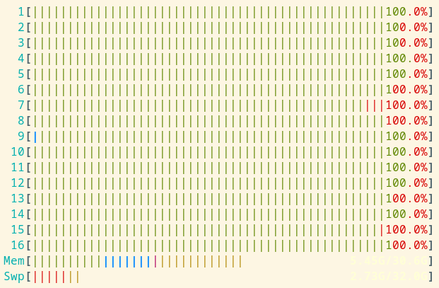
Also note that this approach generalizes to other text-based formats. If you have 10 gigabyte of CSV, you can use Miller for processing. For binary formats, you could use fq if you can find a workable record separator.

The Notebook: Jupyter and Dask

Using GNU parallel is nifty, but for interactive analyses, I prefer Python and Jupyter notebooks. One way of using a notebook with such a large file would be preprocessing it with the parallel magic from the previous section. However, I prefer not having to switch environments while doing data analysis, and using your shell history as documentation is not a sustainable practice (ask me how I know).

Naively reading 9 gigabytes of JSON data with Pandas’ read_json quickly exhausts my 30 gigabytes of RAM, so there is clearly need for some preprocessing. Again, doing this preprocessing in an iterative fashion would be painful if we had to process the whole JSON file again to see our results. We could write some code to only process the first n lines of the JSON file, but I was looking for a more general solution. I’ve mentioned Beam and Flink above, but had no success trying to get a local setup to work.

Dask does what we want: It can partition large datasets, process the partitions in parallel, and merge them back together to get our final output. Let’s create a new Python environment with pipenv, install the necessary dependencies and launch a Jupyter notebook:

pipenv lock
pipenv install jupyterlab dask[distributed] bokeh pandas numpy seaborn
pipenv run jupyter lab

If pipenv is not available, follow the installation instructions to get it set up on your machine. Now, we can get started. We import necessary packages and start a local cluster.

import dask.bag as db
import json
from dask.distributed import Client
client = Client()
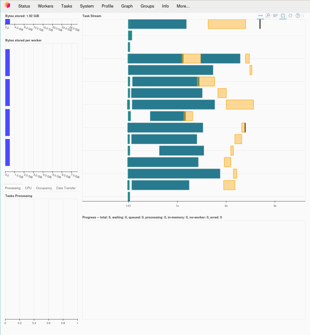
client.dashboard_link

The dashboard link provides a dashboard that shows the activity going on in your local cluster in detail. Every distributed operation we’ll run will use this client. It’s almost like magic!

Now, we can use that local cluster to read our large JSON file into a bag. A bag is an unordered structure, unlike a dataframe, which is ordered and partitioned by its index. It works well with unstructured and nested data, which is why we’re using it here to preprocess our JSON. We can read a text file into a partitioned bag with dask.bag.read_text and the blocksize argument. Note that we’re loading into JSON immediately, as we know the payload is valid JSON.

bag = db.read_text("<file>", blocksize=100 * 1000 * 1000).map(json.loads)
bag

You can get the first few items in the bag with bag.take(5). This will allow you to look at the data and do preprocessing. You can interactively test the preprocessing by adding extra map steps:

bag.map(lambda x: x["artCode"]).take(5)

This will give you the first five article codes in the bag. Note that the function wasn’t called on every element on the bag, only the first five elements, just enough to give us our answer. This is the good thing about using Dask: You’re only running code as needed, which is very useful for finding suitable preprocessing steps.

Once you have a suitable pipeline, you can compute the full data with bag.compute() or turn it into a Dask dataframe with bag.to_dataframe(). Let’s say we wanted to extract the sizes and codes of our subsubarticles from the example above (it’s a very small file, but it’s an illustrative example only). Then, we’d do something like the following:

result = db.read_text("<file>").map(json.loads).map(lambda x: [{"code": z["code"], "size": z["size"]} for y in x["subArts"] for z in y["subSubArts"]])
result.flatten().to_dataframe().compute()

This will run the provided lambda function on each element of the bag, parallel for each partition. flatten will split the list into distinct bag items to allow us to create a non-nested dataframe. Finally, to_dataframe() will convert our data into a Dask dataframe. Calling compute() will execute our pipeline for the whole dataset, which might take a while. However, due to the “laziness” of Dask, you’re able to inspect the intermediate steps in the pipeline interactively (with take() and head()). Additionally, Dask will take care of restarting workers and spilling data to disk if memory is not sufficient. Once we have a Dask dataframe, we can dump it into a more efficient file format like Parquet, which we can then use in the rest of our Python code, either in parallel or in “regular” Pandas.

For 9 gigabytes of JSON, my Laptop was able to execute a data processing pipeline similar to the one above in 50 seconds². Additionally, I was able to build the pipeline in “standard” Python interactively, similar to how I build my jq queries.

Dask has a whole bunch of extra functionality for parallel processing of data, but I hope you’ve gotten a basic understanding of how it works. Compared to jq, you have the full power of Python on your hands, which make it easier to combine data from different sources (files and a database, for example), which is where the shell-based solution starts to struggle.

Fin

I hope you’ve seen that processing large files doesn’t necessarily have to take place in the cloud. A recent laptop or desktop machine is often good enough to run preprocessing and statistics tasks with a bit of tooling³. For me, that tooling consists of jq to answer quick questions during debugging and for deciding on ways to implement features, and Dask to do more involved exploratory data analysis.